Tag: reliability

This post follows up on a previous one where I gave a brief overview of so-called coefficient alpha and recommended against its overuse and traditional attribution to Cronbach. Here, I’m going to cover when to use alpha, also known as tau-equivalent reliability $\rho_T$, and when not to use it, with some demonstrations and plotting in R.

We’re referring to alpha now as tau-equivalent reliability because it’s a more descriptive label that conveys the assumptions supporting its use, again following conventions from Cho (2016).

As I said last time, these concepts aren’t new. They’ve been debated in the literature since the 1940s, with the following conclusions.

1. $\rho_T$ underestimates the actual reliability when the assumptions of tau-equivalence aren’t met, which is likely often the case.
2. $\rho_T$ is not an index of unidimensionality, where multidimensional tests can still produce strong reliability estimates.
3. $\rho_T$ is sensitive to test length, where long tests can produce strong reliability estimates even when items are weakly related to one another.

For each of these points I’ll give a summary and demonstration in R.

Assuming tau equivalence

The main assumption in tau-equivalence is that, in the population, all the items in our test have the same relationship with the underlying construct, which we label tau or $\tau$. This assumption can be expressed in terms of factor loadings or inter-item covariances, where factor loadings are equal or covariances are the same across all pairs of items.

The difference between the tau-equivalent model and the more stringent parallel model is that the latter additionally constrains item variances to be equal whereas these are free to vary with tau-equivalence. The congeneric model is the least restrictive in that it allows both factor loadings (or inter-item covariances) and uniquenesses (item variances) to vary across items.

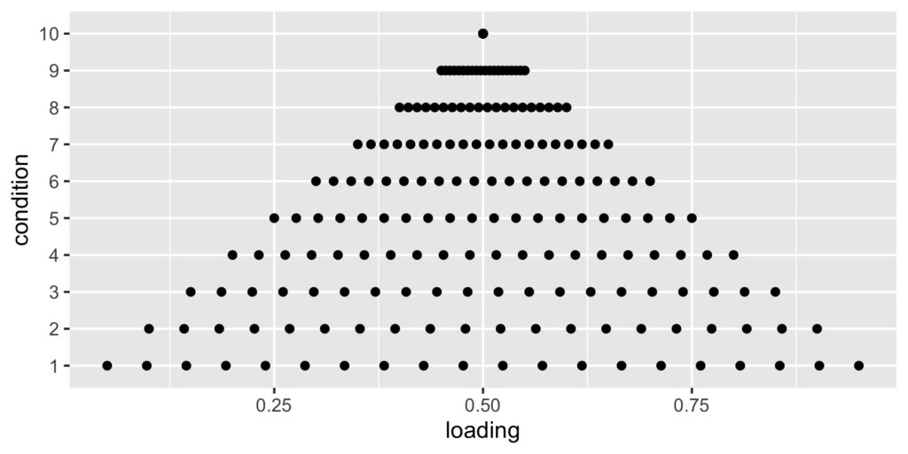
Tau-equivalence is a strong assumption, one that isn’t typically evaluated in practice. Here’s what can happen when it is violated. I’m simulating a test with 20 items that correlate with a single underlying construct to different degrees. At one extreme, the true loadings range from 0.05 to 0.95. At the other extreme, loadings are all 0.50. The mean of the loadings is always 0.50.

This scatterplot shows the loadings per condition as they increase from varying at the bottom, as permitted with the congeneric model, to similar at the top, as required by the tau-equivalent model. Tau-equivalent or coefficient alpha reliability should be most accurate in the top condition, and least accurate in the bottom one.

# Load tidyverse package
# Note the epmr and psych packages are also required
# psych in on CRAN, epmr is on GitHub at talbano/epmr
library("tidyverse")

# Build list of factor loadings for 20 item test
ni <- 20
lm <- lapply(1:10, function(x)
  seq(0 + x * .05, 1 - x * .05, length = ni))

# Visualize the levels of factor loadings
tibble(condition = factor(rep(1:length(lm), each = ni)),
  loading = unlist(lm)) %>%
  ggplot(aes(loading, condition)) + geom_point()

For each of the ten loading conditions, the simulation involved generating 1,000 data sets, each with 200 test takers, and estimating congeneric and tau-equivalent reliability for each. The table below shows the means of the reliability estimates, labeled $\rho_T$ for tau-equivalent and $\rho_C$ for congeneric, per condition, labeled lm.

# Set seed, reps, and output container
set.seed(201210)
reps <- 1000
sim_out <- tibble(lm = numeric(), rep = numeric(),
  omega = numeric(), alpha = numeric())

# Simulate via two loops, j through levels of
# factor loadings, i through reps
for (j in seq_along(lm)) {
  for (i in 1:reps) {
  # Congeneric data are simulated using the psych package
  temp <- psych::sim.congeneric(loads = lm[[j]],
    N = 200, short = F)
  # Alpha and omega are estimated using the epmr package
  sim_out <- bind_rows(sim_out, tibble(lm = j, rep = i,
    omega = epmr::coef_omega(temp$r, sigma = T),
    alpha = epmr::coef_alpha(temp$observed)$alpha))
  }
}

The last column in this table shows the difference between $\rho_T$ and $\rho_C$. Alpha or $\rho_T$ always underestimates omega or $\rho_C$, and the discrepancy is largest in condition lm 1, where the tau-equivalent assumption of equal loadings is most clearly violated. Here, $\rho_T$ underestimates reliability on average by -0.0145. As we progress toward equal factor loadings in lm 10, $\rho_T$ approximates $\rho_C$.

Dimensionality

Tau-equivalent reliability is often misinterpreted as an index of unidimensionality. But $\rho_T$ doesn’t tell us directly how unidimensional our test is. Instead, like parallel and congeneric reliabilities, $\rho_T$ assumes our test measures a single construct or factor. If our items load on multiple distinct dimensions, $\rho_T$ will probably decrease but may still be strong.

Here’s a simple demonstration where I’ll estimate $\rho_T$ for tests simulated to have different amounts of multidimensionality, from completely unidimensional (correlation matrix is all 1s) to completely multidimensional across three factors (correlation matrix with three clusters of 1s). There are nine items.

The next table shows the generating correlation matrix for one of the 11 conditions examined. The three clusters of items (1 through 3, 4 through 6, and 7 through 9) always had perfect correlations, regardless of condition. The remaining off-cluster correlations were fixed within a condition to be 0.1, 0.2, … 1.0. Here, they’re fixed to 0.2. This condition shows strong multidimensionality, within the three factors, and a mild effect from a general factor, with the 0.2.

The simulation again involved generating 1,000 tests, each with 200 test takers, for each condition.

# This will print out the correlation matrix for the
# condition shown in the table above
psych::sim.general(nvar = 9, nfact = 3, g = .2, r = .8)

# Set seed, reps, and output container
set.seed(201211)
reps <- 1000
dim_out <- tibble(dm = numeric(), rep = numeric(),
  alpha = numeric())

# Simulate via two loops, j through levels of
# dimensionality, i through reps
for (j in seq(0, 1, .1)) {
  for (i in 1:reps) {
    # Data are simulated using the psych package
    temp <- psych::sim.general(nvar = 9, nfact = 3,
      g = 1 - j, r = j, n = 200)
    # Estimate alpha with the epmr package
    dim_out <- bind_rows(dim_out, tibble(dm = j, rep = i,
      alpha = epmr::coef_alpha(temp)$alpha))
  }
}

Results below show that mean $\rho_T$ starts out at 1.00 in the unidimensional condition dm1, and decreases to 0.75 in the most multidimensional condition dm11, where the off-cluster correlations were all 0.

The example correlation matrix above corresponds to dm9, showing that a relatively weak general dimension, with prominent group dimensions, still produces mean $\rho_T$ of 0.86.

Test Length

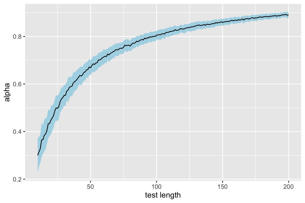
The last demonstration shows how $\rho_T$ gets stronger despite weak factor loadings or weak relationships among items, as test length increases. I’m simulating tests containing 10 to 200 items. For each test length condition, I generate 1,000 tests using a congeneric model with all loadings fixed to 0.20.

# Set seed, reps, and output container
set.seed(201212)
reps <- 100
tim_out <- tibble(tm = numeric(), rep = numeric(),
  alpha = numeric())

# Simulate via two loops, i through levels of
# test length, j through reps
for (j in 10:200) {
  for (i in 1:reps) {
    # Congeneric data are simulated using the psych package
    temp <- psych::sim.congeneric(loads = rep(.2, j),
      N = 200, short = F)
    tim_out <- bind_rows(tim_out, tibble(tm = j, rep = i,
      alpha = epmr::coef_alpha(temp$observed)$alpha))
  }
}

The plot below shows $\rho_T$ on the y-axis for each test length condition on x. The black line captures mean alpha and the ribbon captures the standard deviation over replications for a given condition.

# Summarize with mean and sd of alpha
tim_out %>% group_by(tm) %>%
  summarize(m = mean(alpha), se = sd(alpha)) %>%
  ggplot(aes(tm, m)) + geom_ribbon(aes(ymin = m - se, 
    ymax = m + se), fill = "lightblue") +
  geom_line() + xlab("test length") + ylab("alpha")

Mean $\rho_T$ starts out low at 0.30 for test length 10 items, but surpasses the 0.70 threshold once we hit 56 items. With test length 100 items, we have $\rho_T$ above 0.80, despite having the same weak factor loadings.

When to use tau-equivalent reliability?

These simple demonstrations highlight some of the main limitations of tau-equivalent or alpha reliability. To recap:

1. As the assumption of tau-equivalence will rarely be met in practice, $\rho_T$ will tend to underestimate the actual reliability for our test, though the discrepancy may be small as shown in the first simulation.
2. $\rho_T$ decreases somewhat with departures from unidimensionality, but stays relatively strong even with clear multidimensionality.
3. Test length compensates surprisingly well for low factor loadings and inter-item relationships, producing respectable $\rho_T$ after 50 or so items.

The main benefit of $\rho_T$ is that it’s simpler to calculate than $\rho_C$. Tau-equivalence is thus recommended when circumstances like small sample size make it difficult to fit a congeneric model. We just have to interpret tau-equivalent results with caution, and then plan ahead for a more comprehensive evaluation of reliability.

References

Cho, E. (2016). Making reliability reliable: A systematic approach to reliability coefficients. Organizational Research Methods, 19, 651-682. https://doi.org/10.1177/1094428116656239

References

Greenwald, A. G., Banaji, M. R., & Nosek, B. A. (2015). Statistically small effects of the Implicit Association Test can have societally large effects. Journal of Personality and Social Psychology108(4), 553–561.
Greenwald, A. G., Poehlman, T. A., Uhlmann, E. L., & Banaji, M. R. (2009). Understanding and using the Implicit Association Test: III. Meta-analysis of predictive validity. Journal of Personality and Social Psychology, 97, 17– 41.
Oswald, F. L., Mitchell, G., Blanton, H., Jaccard, J., & Tetlock, P. E. (2013). Predicting ethnic and racial discrimination: A meta-analysis of IAT criterion studies. Journal of Personality and Social Psychology, 105, 171–192.
When to Use Cronbach’s Coefficient Alpha? An Overview and Visualization with R Code
Albano, A. D. (2020). Introduction to Educational and Psychological Measurement Using R. https://thetaminusb.com/intro-measurement-r/
Bandalos, D. L. (2018). Measurement Theory and Applications for the Social Sciences. The Guilford Press.