In this post I’ll answer some frequently asked questions about equating and address common misconceptions about when to use it.
My research on equating mostly examines its application in less than ideal situations, for example, with low stakes, small samples, and shorter tests. I’ve consulted on a variety of operational projects involving equating in formative assessment systems. And I have an R package for observed-score equating, available on CRAN (Albano, 2016).
What is equating?
Equating is a statistical procedure used to create a common measurement scale across two or more forms of a test. The main objective in this procedure is to control statistically for difficulty differences so that scores can be used interchangeably across forms.
In essence, with equating, if some test takers have a more difficult version of a test, they’ll get bonus points. Conversely, if we develop a new test form and discover it to be easier than previous ones, we can also take points away from new test takers. In each case, we’re aiming to establish more fair comparisons. In commercial testing operations, test takers aren’t aware of the score adjustments because they don’t see the raw score scale.
How does equating work?
The input to equating is test scores, whether at the item level or summed across items, and the result is a conversion function that expresses scores from one test form on the scale of the other. Equating works by estimating differences in score distributions, with varying levels of granularity and complexity. If we can assume that the groups assigned to take each form are equivalent or matched with respect to our target construct, any differences in their test score distributions can be attributed to differences in the forms themselves, and our estimate of those differences can be used for score adjustments.
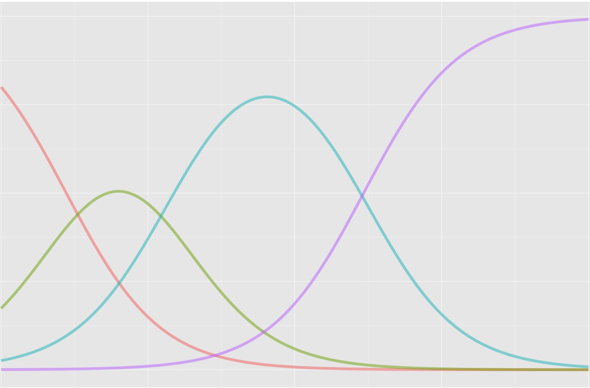
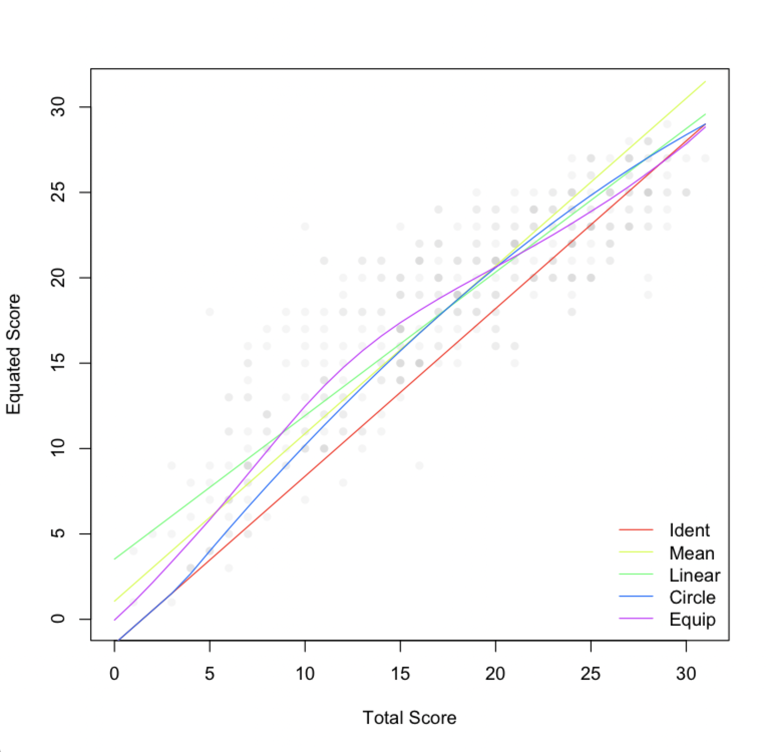
A handful of equating functions are available, increasing in complexity from no equating to item response theory (IRT) functions that incorporate item data. Here’s a summary of the non-IRT functions, also referred to as observed-score equating methods.
Identity equating
Identity equating is no equating, where we assume that score distributions only differ due to noise that we can’t or don’t want to estimate. This is a strong assumption and our potential for bias is maximized. Conversely, we often can’t estimate an equating function because our sample size is too small, so identity becomes the default with insufficient sample sizes (e.g., below 30).
Mean equating
Mean equating applies a constant adjustment to all scores based on the mean difference between score distributions. We’re only estimating means, so sample size requirements are minimized (e.g., 30 or more), but potential for bias is high, where the mean adjustment can be inappropriate for very low or high scoring test takers.
Circle-arc equating
Circle-arc equating is identity equating in the tails of the score scale but mean equating at the mean. It gives us an arching compromise between the two. Assumptions are weaker than with identity, so potential for bias is less and sample size requirements are still low (e.g., 30 or more). Circle-arc also has the practical advantage of automatically truncating the minimum and maximum scores, rather than allowing them to extend beyond the score scale, as can happen with mean or linear equating.
Linear equating
Linear equating adjusts scores via an intercept and slope, as opposed to just the intercept from mean equating. As a result, the score conversion can either grow or shrink from the beginning to the end of the scale. For example, lower scoring test takers could receive a small increase while higher scoring test takers receive a larger one. In this case, test forms differ differentially across the scale. With the additional estimation of the standard deviation (to obtain the slope), potential for bias is decreased but sample sizes should be larger than with the simpler functions (e.g., 100 or more).
Equipercentile equating
Finally, equipercentile equating adjusts for form difficulty differences at each score point, using estimates of the distribution functions for each form. Interpolation and smoothing are used to fill in any gaps, as we’d see with unobserved score points. Because we’re estimating form difficulty differences at the score level, sample size requirements are maximized (e.g., 200 or more), whereas bias is null.
Comparing observed-score functions
I’ve listed the observed-score functions roughly in order of increasing complexity, with identity and mean equating being the simplest and equipercentile being the most complex. The more estimation involved, the more complex the method, and the more test takers we need to support that estimation.
Equipercentile equating is optimal, if you have the data to support it. My advice is to aim for equipercentile equating and then revert to simpler methods if conditions require.

Smoothing
Smoothing is a statistical approach to reducing irregularities in our score distributions prior to equating (called pre-smoothing), or in the score conversion function itself after equating (called post-smoothing). Smoothing is really only necessary with equipercentile equating, as the other observed-score methods incorporate smoothing indirectly via their simplifying assumptions.
I’ve never seen a situation where some amount of smoothing wasn’t necessary prior to implementing equipercentile equating. Usually, it will only help if correctly applied. For the record, I didn’t use smoothing in my first publication on equating (Albano & Rodriguez, 2011) which was a mistake.
Equating vs IRT
Item response theory provides a built-in framework for equating. IRT parameters for test takers and test items are assumed to be invariant, within a linear transformation, over different administration groups and test forms. A linear transformation can put parameters onto the same scale when IRT models are estimated for two separate groups. If we estimate an IRT model using an incomplete data matrix, where not everyone sees all the same items, parameters are directly estimated onto the same scale.
This contrasts with observed-score equating, which mostly ignores item data and instead estimates differences using total scores.
Because IRT can adjust for difficulty differences at the item level, it tends to be more flexible but also more complex than observed-score methods. Sample size requirements vary by IRT model (e.g., from 100 to 1000 or more).
Equating vs linking
People use different terms to label the process of estimating conversions from one score distribution to another. There are detailed taxonomies outlining when the conversion should be referred to as equating vs linking vs scaling (see Kolen & Brennan, 2014). Linking is the most generic term, though equating is more commonly used.
In the end, it’s how we obtain data for the score conversions, through study design and test development, that determines the type of score conversion we get and how we can interpret it. The actual functions themselves change little or not at all across a taxonomy.
When to use equating?
The simple answer here is, we should always use equating as long as our sample size and study design support it. The danger in equating is that we might introduce more error into score interpretations because of inaccurate estimation. If our sample sizes are too small (e.g., below 30) or our study design lacks control or consistency (e.g., non-random assignment to test forms), equating may be problematic.
What about sample size?
Although simpler equating functions require smaller sample sizes, there are no clear guidelines regarding how many test takers are needed, mostly because sample size requirements depend on score scale length (the number of score points, typically based on the length of the test) and our tolerance for standard error and bias.
Score scale length is often not considered in planning an equating study, but should be. A sample size of 100 goes a long way with a limited score scale (e.g., 10 points) but is less optimal with a longer one (e.g., 50 points). In the former case, all our score points will likely be represented well making it more feasible to use complex equating methods, whereas in the latter case our data become more sparse and simpler methods may be needed.
References
Albano, A. D. (2016). equate: An R package for observed-score linking and equating. Journal of Statistical Software, 74(8), 1–36.
Albano, A. D., & Rodriguez, M. C. (2012). Statistical equating with measures of oral reading fluency. Journal of School Psychology, 50, 43–59.
Kolen, M. J., & Brennan, R. L. (2014). Test equating, scaling, and linking. New York, NY: Springer.