When to Use Cronbach’s Coefficient Alpha? An Overview and Visualization with R Code

This post follows up on a previous one where I gave a brief overview of so-called coefficient alpha and recommended against its overuse and traditional attribution to Cronbach. Here, I’m going to cover when to use alpha, also known as tau-equivalent reliability $\rho_T$, and when not to use it, with some demonstrations and plotting in R.

We’re referring to alpha now as tau-equivalent reliability because it’s a more descriptive label that conveys the assumptions supporting its use, again following conventions from Cho (2016).

As I said last time, these concepts aren’t new. They’ve been debated in the literature since the 1940s, with the following conclusions.

  1. $\rho_T$ underestimates the actual reliability when the assumptions of tau-equivalence aren’t met, which is likely often the case.
  2. $\rho_T$ is not an index of unidimensionality, where multidimensional tests can still produce strong reliability estimates.
  3. $\rho_T$ is sensitive to test length, where long tests can produce strong reliability estimates even when items are weakly related to one another.

For each of these points I’ll give a summary and demonstration in R.

Assuming tau equivalence

The main assumption in tau-equivalence is that, in the population, all the items in our test have the same relationship with the underlying construct, which we label tau or $\tau$. This assumption can be expressed in terms of factor loadings or inter-item covariances, where factor loadings are equal or covariances are the same across all pairs of items.

The difference between the tau-equivalent model and the more stringent parallel model is that the latter additionally constrains item variances to be equal whereas these are free to vary with tau-equivalence. The congeneric model is the least restrictive in that it allows both factor loadings (or inter-item covariances) and uniquenesses (item variances) to vary across items.

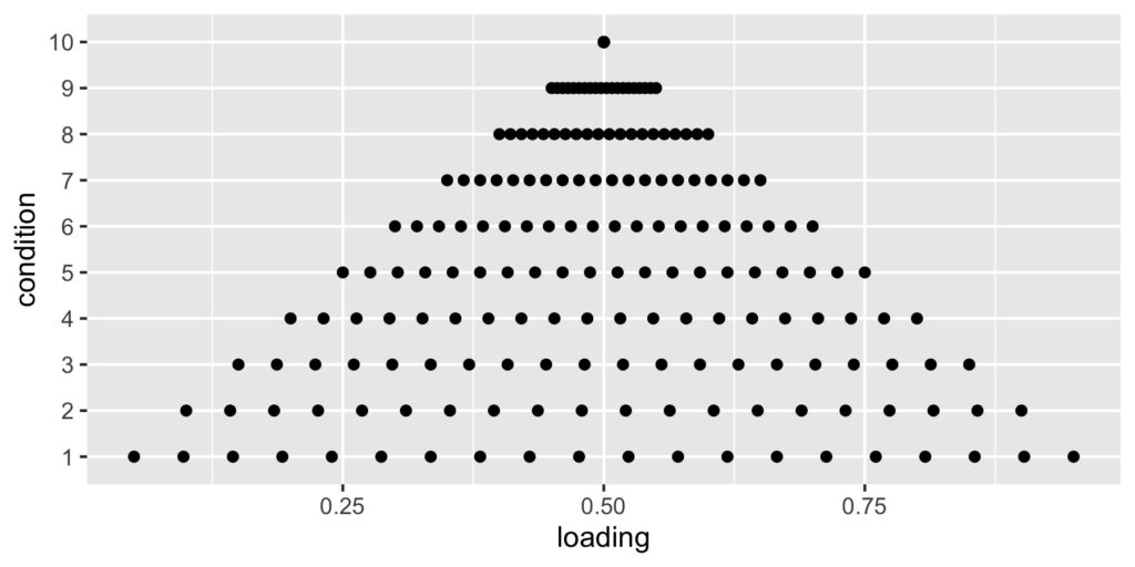
Tau-equivalence is a strong assumption, one that isn’t typically evaluated in practice. Here’s what can happen when it is violated. I’m simulating a test with 20 items that correlate with a single underlying construct to different degrees. At one extreme, the true loadings range from 0.05 to 0.95. At the other extreme, loadings are all 0.50. The mean of the loadings is always 0.50.

This scatterplot shows the loadings per condition as they increase from varying at the bottom, as permitted with the congeneric model, to similar at the top, as required by the tau-equivalent model. Tau-equivalent or coefficient alpha reliability should be most accurate in the top condition, and least accurate in the bottom one.

# Load tidyverse package
# Note the epmr and psych packages are also required
# psych in on CRAN, epmr is on GitHub at talbano/epmr
library("tidyverse")

# Build list of factor loadings for 20 item test
ni <- 20
lm <- lapply(1:10, function(x)
  seq(0 + x * .05, 1 - x * .05, length = ni))

# Visualize the levels of factor loadings
tibble(condition = factor(rep(1:length(lm), each = ni)),
  loading = unlist(lm)) %>%
  ggplot(aes(loading, condition)) + geom_point()
Factor loadings across ten range conditions

For each of the ten loading conditions, the simulation involved generating 1,000 data sets, each with 200 test takers, and estimating congeneric and tau-equivalent reliability for each. The table below shows the means of the reliability estimates, labeled $\rho_T$ for tau-equivalent and $\rho_C$ for congeneric, per condition, labeled lm.

# Set seed, reps, and output container
set.seed(201210)
reps <- 1000
sim_out <- tibble(lm = numeric(), rep = numeric(),
  omega = numeric(), alpha = numeric())

# Simulate via two loops, j through levels of
# factor loadings, i through reps
for (j in seq_along(lm)) {
  for (i in 1:reps) {
  # Congeneric data are simulated using the psych package
  temp <- psych::sim.congeneric(loads = lm[[j]],
    N = 200, short = F)
  # Alpha and omega are estimated using the epmr package
  sim_out <- bind_rows(sim_out, tibble(lm = j, rep = i,
    omega = epmr::coef_omega(temp$r, sigma = T),
    alpha = epmr::coef_alpha(temp$observed)$alpha))
  }
}
lm $\rho_T$ $\rho_C$ diff
1 0.8662 0.8807 -0.0145
2 0.8663 0.8784 -0.0121
3 0.8665 0.8757 -0.0093
4 0.8668 0.8735 -0.0067
5 0.8673 0.8720 -0.0047
6 0.8673 0.8706 -0.0032
7 0.8680 0.8701 -0.0020
8 0.8688 0.8699 -0.0011
9 0.8686 0.8692 -0.0006
10 0.8681 0.8685 -0.0004
Mean reliabilities by condition

The last column in this table shows the difference between $\rho_T$ and $\rho_C$. Alpha or $\rho_T$ always underestimates omega or $\rho_C$, and the discrepancy is largest in condition lm 1, where the tau-equivalent assumption of equal loadings is most clearly violated. Here, $\rho_T$ underestimates reliability on average by -0.0145. As we progress toward equal factor loadings in lm 10, $\rho_T$ approximates $\rho_C$.

Dimensionality

Tau-equivalent reliability is often misinterpreted as an index of unidimensionality. But $\rho_T$ doesn’t tell us directly how unidimensional our test is. Instead, like parallel and congeneric reliabilities, $\rho_T$ assumes our test measures a single construct or factor. If our items load on multiple distinct dimensions, $\rho_T$ will probably decrease but may still be strong.

Here’s a simple demonstration where I’ll estimate $\rho_T$ for tests simulated to have different amounts of multidimensionality, from completely unidimensional (correlation matrix is all 1s) to completely multidimensional across three factors (correlation matrix with three clusters of 1s). There are nine items.

The next table shows the generating correlation matrix for one of the 11 conditions examined. The three clusters of items (1 through 3, 4 through 6, and 7 through 9) always had perfect correlations, regardless of condition. The remaining off-cluster correlations were fixed within a condition to be 0.1, 0.2, … 1.0. Here, they’re fixed to 0.2. This condition shows strong multidimensionality, within the three factors, and a mild effect from a general factor, with the 0.2.

i1 i2 i3 i4 i5 i6 i7 i8 i9
i1 1.0 1.0 1.0 0.2 0.2 0.2 0.2 0.2 0.2
i2 1.0 1.0 1.0 0.2 0.2 0.2 0.2 0.2 0.2
i3 1.0 1.0 1.0 0.2 0.2 0.2 0.2 0.2 0.2
i4 0.2 0.2 0.2 1.0 1.0 1.0 0.2 0.2 0.2
i5 0.2 0.2 0.2 1.0 1.0 1.0 0.2 0.2 0.2
i6 0.2 0.2 0.2 1.0 1.0 1.0 0.2 0.2 0.2
i7 0.2 0.2 0.2 0.2 0.2 0.2 1.0 1.0 1.0
i8 0.2 0.2 0.2 0.2 0.2 0.2 1.0 1.0 1.0
i9 0.2 0.2 0.2 0.2 0.2 0.2 1.0 1.0 1.0
Correlation matrix showing some multidimensionality

The simulation again involved generating 1,000 tests, each with 200 test takers, for each condition.

# This will print out the correlation matrix for the
# condition shown in the table above
psych::sim.general(nvar = 9, nfact = 3, g = .2, r = .8)

# Set seed, reps, and output container
set.seed(201211)
reps <- 1000
dim_out <- tibble(dm = numeric(), rep = numeric(),
  alpha = numeric())

# Simulate via two loops, j through levels of
# dimensionality, i through reps
for (j in seq(0, 1, .1)) {
  for (i in 1:reps) {
    # Data are simulated using the psych package
    temp <- psych::sim.general(nvar = 9, nfact = 3,
      g = 1 - j, r = j, n = 200)
    # Estimate alpha with the epmr package
    dim_out <- bind_rows(dim_out, tibble(dm = j, rep = i,
      alpha = epmr::coef_alpha(temp)$alpha))
  }
}

Results below show that mean $\rho_T$ starts out at 1.00 in the unidimensional condition dm1, and decreases to 0.75 in the most multidimensional condition dm11, where the off-cluster correlations were all 0.

The example correlation matrix above corresponds to dm9, showing that a relatively weak general dimension, with prominent group dimensions, still produces mean $\rho_T$ of 0.86.

dm1 dm2 dm3 dm4 dm5 dm6 dm7 dm8 dm9 dm10 dm11
1.000.99 0.98 0.97 0.96 0.94 0.92 0.89 0.86 0.81 0.75
Mean alphas for 11 conditions of multidimensionality

Test Length

The last demonstration shows how $\rho_T$ gets stronger despite weak factor loadings or weak relationships among items, as test length increases. I’m simulating tests containing 10 to 200 items. For each test length condition, I generate 1,000 tests using a congeneric model with all loadings fixed to 0.20.

# Set seed, reps, and output container
set.seed(201212)
reps <- 100
tim_out <- tibble(tm = numeric(), rep = numeric(),
  alpha = numeric())

# Simulate via two loops, i through levels of
# test length, j through reps
for (j in 10:200) {
  for (i in 1:reps) {
    # Congeneric data are simulated using the psych package
    temp <- psych::sim.congeneric(loads = rep(.2, j),
      N = 200, short = F)
    tim_out <- bind_rows(tim_out, tibble(tm = j, rep = i,
      alpha = epmr::coef_alpha(temp$observed)$alpha))
  }
}

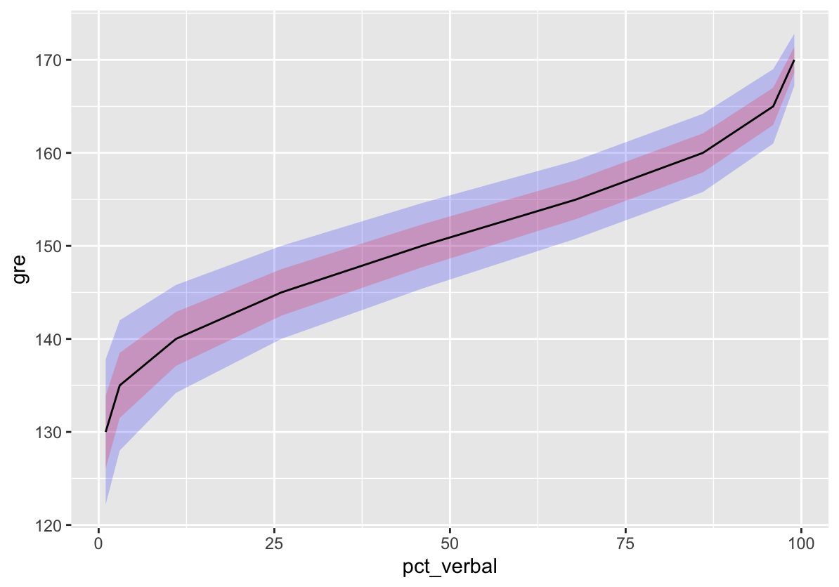
The plot below shows $\rho_T$ on the y-axis for each test length condition on x. The black line captures mean alpha and the ribbon captures the standard deviation over replications for a given condition.

# Summarize with mean and sd of alpha
tim_out %>% group_by(tm) %>%
  summarize(m = mean(alpha), se = sd(alpha)) %>%
  ggplot(aes(tm, m)) + geom_ribbon(aes(ymin = m - se, 
    ymax = m + se), fill = "lightblue") +
  geom_line() + xlab("test length") + ylab("alpha")
Alpha as a function of test length when factor loadings are fixed at 0.20

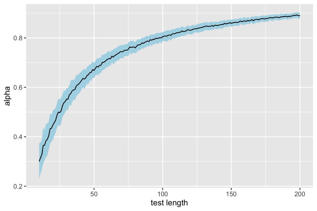
Mean $\rho_T$ starts out low at 0.30 for test length 10 items, but surpasses the 0.70 threshold once we hit 56 items. With test length 100 items, we have $\rho_T$ above 0.80, despite having the same weak factor loadings.

When to use tau-equivalent reliability?

These simple demonstrations highlight some of the main limitations of tau-equivalent or alpha reliability. To recap:

  1. As the assumption of tau-equivalence will rarely be met in practice, $\rho_T$ will tend to underestimate the actual reliability for our test, though the discrepancy may be small as shown in the first simulation.
  2. $\rho_T$ decreases somewhat with departures from unidimensionality, but stays relatively strong even with clear multidimensionality.
  3. Test length compensates surprisingly well for low factor loadings and inter-item relationships, producing respectable $\rho_T$ after 50 or so items.

The main benefit of $\rho_T$ is that it’s simpler to calculate than $\rho_C$. Tau-equivalence is thus recommended when circumstances like small sample size make it difficult to fit a congeneric model. We just have to interpret tau-equivalent results with caution, and then plan ahead for a more comprehensive evaluation of reliability.

References

Cho, E. (2016). Making reliability reliable: A systematic approach to reliability coefficients. Organizational Research Methods, 19, 651-682. https://doi.org/10.1177/1094428116656239

An Intro to Test Score Equating, What it is, When to Use it

In this post I’ll answer some frequently asked questions about equating and address common misconceptions about when to use it.

My research on equating mostly examines its application in less than ideal situations, for example, with low stakes, small samples, and shorter tests. I’ve consulted on a variety of operational projects involving equating in formative assessment systems. And I have an R package for observed-score equating, available on CRAN (Albano, 2016).

What is equating?

Equating is a statistical procedure used to create a common measurement scale across two or more forms of a test. The main objective in this procedure is to control statistically for difficulty differences so that scores can be used interchangeably across forms.

In essence, with equating, if some test takers have a more difficult version of a test, they’ll get bonus points. Conversely, if we develop a new test form and discover it to be easier than previous ones, we can also take points away from new test takers. In each case, we’re aiming to establish more fair comparisons. In commercial testing operations, test takers aren’t aware of the score adjustments because they don’t see the raw score scale.

How does equating work?

The input to equating is test scores, whether at the item level or summed across items, and the result is a conversion function that expresses scores from one test form on the scale of the other. Equating works by estimating differences in score distributions, with varying levels of granularity and complexity. If we can assume that the groups assigned to take each form are equivalent or matched with respect to our target construct, any differences in their test score distributions can be attributed to differences in the forms themselves, and our estimate of those differences can be used for score adjustments.

A handful of equating functions are available, increasing in complexity from no equating to item response theory (IRT) functions that incorporate item data. Here’s a summary of the non-IRT functions, also referred to as observed-score equating methods.

Identity equating

Identity equating is no equating, where we assume that score distributions only differ due to noise that we can’t or don’t want to estimate. This is a strong assumption and our potential for bias is maximized. Conversely, we often can’t estimate an equating function because our sample size is too small, so identity becomes the default with insufficient sample sizes (e.g., below 30).

Mean equating

Mean equating applies a constant adjustment to all scores based on the mean difference between score distributions. We’re only estimating means, so sample size requirements are minimized (e.g., 30 or more), but potential for bias is high, where the mean adjustment can be inappropriate for very low or high scoring test takers.

Circle-arc equating

Circle-arc equating is identity equating in the tails of the score scale but mean equating at the mean. It gives us an arching compromise between the two. Assumptions are weaker than with identity, so potential for bias is less and sample size requirements are still low (e.g., 30 or more). Circle-arc also has the practical advantage of automatically truncating the minimum and maximum scores, rather than allowing them to extend beyond the score scale, as can happen with mean or linear equating.

Linear equating

Linear equating adjusts scores via an intercept and slope, as opposed to just the intercept from mean equating. As a result, the score conversion can either grow or shrink from the beginning to the end of the scale. For example, lower scoring test takers could receive a small increase while higher scoring test takers receive a larger one. In this case, test forms differ differentially across the scale. With the additional estimation of the standard deviation (to obtain the slope), potential for bias is decreased but sample sizes should be larger than with the simpler functions (e.g., 100 or more).

Equipercentile equating

Finally, equipercentile equating adjusts for form difficulty differences at each score point, using estimates of the distribution functions for each form. Interpolation and smoothing are used to fill in any gaps, as we’d see with unobserved score points. Because we’re estimating form difficulty differences at the score level, sample size requirements are maximized (e.g., 200 or more), whereas bias is null.

Comparing observed-score functions

I’ve listed the observed-score functions roughly in order of increasing complexity, with identity and mean equating being the simplest and equipercentile being the most complex. The more estimation involved, the more complex the method, and the more test takers we need to support that estimation.

Equipercentile equating is optimal, if you have the data to support it. My advice is to aim for equipercentile equating and then revert to simpler methods if conditions require.

Raw (black) vs smoothed (red) score distributions

Smoothing

Smoothing is a statistical approach to reducing irregularities in our score distributions prior to equating (called pre-smoothing), or in the score conversion function itself after equating (called post-smoothing). Smoothing is really only necessary with equipercentile equating, as the other observed-score methods incorporate smoothing indirectly via their simplifying assumptions.

I’ve never seen a situation where some amount of smoothing wasn’t necessary prior to implementing equipercentile equating. Usually, it will only help if correctly applied. For the record, I didn’t use smoothing in my first publication on equating (Albano & Rodriguez, 2011) which was a mistake.

Equating vs IRT

Item response theory provides a built-in framework for equating. IRT parameters for test takers and test items are assumed to be invariant, within a linear transformation, over different administration groups and test forms. A linear transformation can put parameters onto the same scale when IRT models are estimated for two separate groups. If we estimate an IRT model using an incomplete data matrix, where not everyone sees all the same items, parameters are directly estimated onto the same scale.

This contrasts with observed-score equating, which mostly ignores item data and instead estimates differences using total scores.

Because IRT can adjust for difficulty differences at the item level, it tends to be more flexible but also more complex than observed-score methods. Sample size requirements vary by IRT model (e.g., from 100 to 1000 or more).

Equating vs linking

People use different terms to label the process of estimating conversions from one score distribution to another. There are detailed taxonomies outlining when the conversion should be referred to as equating vs linking vs scaling (see Kolen & Brennan, 2014). Linking is the most generic term, though equating is more commonly used.

In the end, it’s how we obtain data for the score conversions, through study design and test development, that determines the type of score conversion we get and how we can interpret it. The actual functions themselves change little or not at all across a taxonomy.

When to use equating?

The simple answer here is, we should always use equating as long as our sample size and study design support it. The danger in equating is that we might introduce more error into score interpretations because of inaccurate estimation. If our sample sizes are too small (e.g., below 30) or our study design lacks control or consistency (e.g., non-random assignment to test forms), equating may be problematic.

What about sample size?

Although simpler equating functions require smaller sample sizes, there are no clear guidelines regarding how many test takers are needed, mostly because sample size requirements depend on score scale length (the number of score points, typically based on the length of the test) and our tolerance for standard error and bias.

Score scale length is often not considered in planning an equating study, but should be. A sample size of 100 goes a long way with a limited score scale (e.g., 10 points) but is less optimal with a longer one (e.g., 50 points). In the former case, all our score points will likely be represented well making it more feasible to use complex equating methods, whereas in the latter case our data become more sparse and simpler methods may be needed.

References

Albano, A. D. (2016). equate: An R package for observed-score linking and equating. Journal of Statistical Software, 74(8), 1–36.

Albano, A. D., & Rodriguez, M. C. (2012). Statistical equating with measures of oral reading fluency. Journal of School Psychology, 50, 43–59.

Kolen, M. J., & Brennan, R. L. (2014). Test equating, scaling, and linking. New York, NY: Springer.

Article in Frontiers in Education

My colleagues and I recently published an open-access article in Frontiers in Education titled Contextual Interference Effects in Early Assessment: Evaluating the Psychometric Benefits of Item Interleaving. We looked at how interleaving as opposed to blocking items by task affects the psychometric properties of a test.

Here’s the abstract and link to the full text.

https://www.frontiersin.org/articles/10.3389/feduc.2020.00133/full

Research has shown that the context of practice tasks can have a significant impact on learning, with long-term retention and transfer improving when tasks of different types are mixed by interleaving (abcabcabc) compared with grouping together in blocks (aaabbbccc). This study examines the influence of context via interleaving from a psychometric perspective, using educational assessments designed for early childhood. An alphabet knowledge measure consisting of four types of tasks (finding, orienting, selecting, and naming letters) was administered in two forms, one with items blocked by task, and the other with items interleaved and rotating from one task to the next by item. The interleaving of tasks, and thereby the varying of item context, had a negligible impact on mean performance, but led to stronger internal consistency reliability as well as improved item discrimination. Implications for test design and student engagement in educational measurement are discussed.

The plots below show item difficulty (on the left) and discrimination (right) for 20 items. Plotting characters represent the task for each item, abbreviated as F, O, S, and N (letter finding, orienting, selecting, and naming, respectively), with results from the blocked administration on the x-axis and interleaving on the y-axis.

Our sample sizes (50 for blocked and 55 for interleaving) didn’t support item-level comparisons, but the overall trends are still interesting. Item difficulties don’t appear to change consistently but discriminations do seem to increase overall for interleaved.


Thoughts on Cronbach’s Coefficient Alpha

I have a few thoughts to share on coefficient alpha, the ubiquitous and frequently misused psychometric index of internal consistency reliability. These thoughts aren’t new, people have thought and written about them before (references below), but they’re worth repeating, as the majority of those who cite Cronbach (1951) seem to be unaware that:

  1. alpha is not the only or best measure of internal consistency reliability,
  2. strong alpha does not indicate unidimensionality or a single underlying construct, and
  3. Cronbach ultimately regretted that his alpha became the preferred index.

What is alpha?

Coefficient alpha indexes the extent to which the components of a scale function together in a consistent way. Higher alpha (closer to 1) vs lower alpha (closer to 0) means higher vs lower consistency.

The most common use of alpha is with items or questions within an educational or psychological test, where the composite is a total summed score. If we can determine that a set of test items is internally consistent, with a strong alpha, we can be more confident that a total on our test will provide a cohesive summary of performance across items. Low alpha suggests we shouldn’t combine our items by summing. In this case, the total is expected to have less consistent meaning.

Alpha estimates reliability using the average of the relationships among scored items. This is contrasted with the overall variability for the composite, based on the variance $\sigma^2_X$ of the total score $X$. If we find the covariance for each distinct item pair $X_j$ and $X_{j’}$ and then get the mean as $\bar{\sigma}_{X_jX_{j’}}$, we have

$$\rho_T = J^2\frac{\bar{\sigma}_{X_jX_{j’}}}{\sigma^2_X}$$

where $J$ is the number of items in the test. I’m using the label $\rho_T$ instead of alpha, where the $T$ denotes tau-equivalent reliability, following conventions from Cho (2016).

Alpha isn’t necessarily best

There are lots of papers outlining alpha as one among a variety of options for estimating reliability with scores from a single administration of a test. See the Wikipedia entries on tau-equivalent reliability, which encompasses alpha, and congeneric reliability for accessible summaries.

Most often, alpha is contrasted with what are called congeneric reliability estimates. A simple example is the ratio of the squared sum of standardized factor loadings $(\sum\lambda)^2$ from a unidimensional model, to total variance, or

$$\rho_C = \frac{(\sum\lambda)^2}{\sigma^2_X}.$$

Congeneric reliability indices are often recommended because they have less strict assumptions than tau-equivalent ones like alpha.

  • Tau-equivalent reliability, including alpha, allows individual item variances to differ, but assumes unidimensionality as well as equal inter-item covariances in the population.
  • Congeneric reliability allows individual item variances and inter-item covariances to differ, and only assumes unidimensionality in the population.

When the stricter assumptions of alpha aren’t met, which is typically the case in practice, alpha will underestimate and/or misrepresent reliability.

Cronbach and Schavelson (2004) recommended the more comprehensive generalizability theory in place of a narrow focus on alpha. More direct critiques of alpha include Sijtsma (2009), with a response from Revelle and Zinbarg (2009), and McNeish (2017), with a response from Raykov and Marcoulides (2019). Cho (2016) proposes a new perspective on the relationships among alpha and other reliability coefficients, as well as a new naming convention.

Alpha is not a direct measure of unidimensionality

A common misconception is that strong alpha is evidence of unidimensionality, that is, a single construct or factor underlying a set of items. The literature has thoroughly addressed this point, so I’ll just summarize by saying that

  • alpha assumes undimensionality, and works best when it’s present, but
  • strong alpha does not confirm that a scale is unidimensional, instead, alpha can be strong with a multidimensional scale.

These and related points have led some (e.g., Sijtsma, 2009) to recommend against the term internal consistency reliability because it suggests that alpha reflects the internal structure of the test, which it does not do, at least not consistently (Cortina, 1993).

Cronbach’s comments on alpha

Cronbach (1951) didn’t invent tau-equivalent reliability or the foundations for what would become coefficient alpha. Instead, he gave an existing coefficient an accessible derivation, as well as a catchy, seemingly preeminent greek label. The same or similar formulations were available in publications predating Cronbach’s article (for a summary, see the tau-equivalent reliability Wikipedia entry). This isn’t something Cronbach tried to hide, and it’s not necessarily a criticism of his work, but most people are unaware of these details and we’ve gotten carried away with the attribution, a fact that Cronbach himself lamented (2004, p 397):

To make so much use of an easily calculated translation of a well-established formula scarcely justifies the fame it has brought me. It is an embarrassment to me that the formula became conventionally known as Cronbach’s alpha.

I suggest we refer to alpha simply as coefficient alpha, or use a more specific term like tau-equivalent reliability. If we need a reference, we should use something more recent, comprehensive, and accessible, like one of the papers mentioned above or a measurement textbook (e.g., Albano, 2020; Bandalos, 2018). I also recommend considering alternative indices, and being more thoughtful about the choice. This may go against the grain, but it makes sense given the history and research.

If abandoning the Cronbach moniker isn’t rebellious enough for you, I also recommend against the omnipresent Likert scale for similar reasons which I’ll get into later.

[Update May 26, 2020: revised the formulas and added references.]

References

Albano, A. D. (2020). Introduction to Educational and Psychological Measurement Using R. https://thetaminusb.com/intro-measurement-r/

Bandalos, D. L. (2018). Measurement Theory and Applications for the Social Sciences. The Guilford Press.

Cho, E. (2016). Making reliability reliable: A systematic approach to reliability coefficients. Organizational Research Methods, 19, 651-682. https://doi.org/10.1177/1094428116656239

Cortina, J. M. (1993). What is coefficient alpha? An examination of theory and applications. Journal of Applied Psychology, 78, 98-104.

Cronbach, L.J. (1951). Coefficient alpha and the internal structure of tests. Psychometrika, 16, 297–334. https://doi.org/10.1007/BF02310555

Cronbach, L. J., & Shavelson, R. J. (2004). My current thoughts on coefficient alpha and successor procedures. Educational and Psychological Measurement, 64, 391–418. https://doi.org/10.1177/0013164404266386

McNeish, D. (2017). Thanks coefficient alpha, we’ll take it from here. Psychological Methods, 23, 412–433. https://doi.org/10.1037/met0000144

Raykov, T., & Marcoulides, G. A. (2017). Thanks coefficient alpha, we still need you! Educational and Psychological Measurement, 79, 200–210. https://doi.org/10.1177/0013164417725127

Revelle, W., & Zinbarg, R. E. (2009). Coefficients alpha, beta, omega, and the glb: Comments on Sijtsma. Psychometrika, 74, 145–154. https://doi.org/10.1007/s11336-008-9102-z

Sijtsma, K. (2009). On the use, the misuse, and the very limited usefulness of Cronbach’s alpha. Psychometrika, 74, 107–120. https://doi.org/10.1007/s11336-008-9101-0

Article in Frontiers in Computer Science

A colleague and I recently published an open-access article in Frontiers, titled Development and Evaluation of the Nebraska Assessment of Computing Knowledge. Abstract and link to full text are below.

One way to increase the quality of computing education research is to increase the quality of the measurement tools that are available to researchers, especially measures of students’ knowledge and skills. This paper represents a step toward increasing the number of available thoroughly-evaluated tests that can be used in computing education research by evaluating the psychometric properties of a multiple-choice test designed to differentiate undergraduate students in terms of their mastery of foundational computing concepts. Classical test theory and item response theory analyses are reported and indicate that the test is a reliable, psychometrically-sound instrument suitable for research with undergraduate students. Limitations and the importance of using standardized measures of learning in education research are discussed.

https://www.frontiersin.org/articles/10.3389/fcomp.2020.00011/full

Teaching and Learning Online During the Lockdown

Here are some pointers on transitioning college coursework to online delivery. I’m not an expert on the topic, and have never done it under threat of a pandemic, but I did figure out the basics through trial and error while teaching at Nebraska. For a few years I offered my intro measurement course via traditional in-person instruction in the spring semester and then online in the summer. Here’s what I learned.

Use technology to strengthen the online experience, not mimic the physical one

There’s no way to replicate the in-person experience from a distance, and that shouldn’t be the goal. Instead, we should become familiar with the available technology and consider how it can best be used to support the course objectives. When meeting in the same physical space, we’re hearing the same sounds and breathing the same air. We’re often seeing detailed facial expressions and picking up on subtle cues. None of this can be captured through a pixelated video call or static discussion post.

The learning environment is different online, and we should chose our technology based on its strengths.

  • Video or conference calls are good for presentations and lecture, and for efficiently communicating general information to a large audience.
  • Recorded presentations are good for presenting material in depth, since students can review as many times as needed. In this way, recordings can sometimes be more effective than live lecture, as exemplified in the flipped classroom movement.
  • Discussion forums can give everyone a voice, and are especially useful for encouraging thoughtful comments and questions that may be difficult for students to generate impromptu in class.

Prioritize accessibility

Providing all students with effective access to course materials is paramount across delivery modes, but we may take it for granted when switching to online that a given technology works equally well for all students. Some questions to consider.

  • Do all students have regular high-speed internet access as well as uninterrupted access to the required computing technology at home?
  • Does an increased digital reading load differentially impact multilingual students or students with visual impairment?
  • Do online formats enable less formal communication and the use of jargon that may be unfamiliar to international students?
  • Is getting to a testing center feasible for all students?

Facilitate independent study

My online courses involve much more independent work, as online allows students to proceed at their own pace. I expect this will be especially helpful when we’re on lockdown with extra responsibilities and different schedules at home. The trade-off with increased independence is decreased collaboration and less structure in pacing. It’s difficult to work together on an assignment or share the scoring key if some students haven’t completed it.

Here’s how my courses tend to work.

  • I try to post all of the course materials, slides, readings, assignments, rubrics, due dates, within the first week of class.
  • Group work is challenging from a distance, especially when students have never met in person and when they have very different schedules. I try to simplify it or avoid it online.
  • If I do have group assignments, they’re either brief or pushed to the end of the course. Students know about them early on, so they can plan accordingly. And students must commit to being caught up by the time a group assignment is given.
  • I still have a schedule for readings and assignments, but some of the due dates are flexible. I’ve found that the majority of students follow the suggested pacing, but some take advantage of the flexibility, especially in my summer courses. It might make sense to have some hard deadlines, with softer ones in between.

Lockdown considerations

UC Davis has provided lots of resources for teaching and learning during the lockdown, which I expect will extend into summer and may impact fall instruction as well. Many of these generalize to instruction in any college course. This link organizes most of what Davis has provided.

https://keepteaching.ucdavis.edu

Visualizing Conditional Standard Error in the GRE

Below is some R code for visualizing measurement error across the GRE score scale, plotted against percentiles. Data come from an ETS report at https://www.ets.org/s/gre/pdf/gre_guide.pdf.

The plot shows conditional standard error of measurement (SEM) for GRE verbal scores. SEM is the expected average variability in scores attributable to random error in the measurement process. For details, see my last post.

Here, the SEM is conditional on GRE score, with more error evident at lower verbal scores, and less at higher scores where measurement is more precise. As with other forms of standard error, the SEM can be used to build confidence intervals around an estimate. The plot has ribbons for 68% and 95% confidence intervals, based on +/- 1 and 2 SEM.

# Load ggplot2 package
library("ggplot2")

# Put percentiles into data frame, pasting from ETS
# report Table 1B
pct <- data.frame(gre = 170:130,
matrix(c(99, 96, 99, 95, 98, 93, 98, 90, 97, 89,
  96, 86, 94, 84, 93, 82, 90, 79, 88, 76, 86, 73,
  83, 70, 80, 67, 76, 64, 73, 60, 68, 56, 64, 53,
  60, 49, 54, 45, 51, 41, 46, 37, 41, 34, 37, 30,
  33, 26, 29, 23, 26, 19, 22, 16, 19, 13, 16, 11,
  14, 9, 11, 7, 9, 6, 8, 4, 6, 3, 4, 2, 3, 2, 2,
  1, 2, 1, 1, 1, 1, 1, 1, 1),
  nrow = 41, byrow = T))

# Add variable names
colnames(pct)[2:3] <- c("pct_verbal", "pct_quant")

# Subset and add conditional SEM from Table 5E
sem <- data.frame(pct[c(41, seq(36, 1, by = -5)), ],
  sem_verbal = c(3.9, 3.5, 2.9, 2.5, 2.3, 2.1, 2.1,
    2.0, 1.4),
  sem_quant = c(3.5, 2.9, 2.4, 2.2, 2.1, 2.0, 2.1,
    2.1, 1.0),
  row.names = NULL)

# Plot percentiles on x and GRE on y with
# error ribbons
ggplot(sem, aes(pct_verbal, gre)) +
  geom_ribbon(aes(ymin = gre - sem_verbal * 2,
    ymax = gre + sem_verbal * 2),
    fill = "blue", alpha = .2) +
  geom_ribbon(aes(ymin = gre - sem_verbal,
    ymax = gre + sem_verbal),
    fill = "red", alpha = .2) +
  geom_line()

Confidence Intervals in Measurement vs Political Polls

In class this week we covered reliability and went through some examples of how measurement error, the opposite of reliability, can be converted into a standard error for building confidence intervals (CI) around test scores. Students are often surprised to learn that, despite a moderate to strong reliability coefficient, a test can still introduce an unsettling amount of error into results.

Measurement

Here’s an example from testing before I get to error in political polling. The GRE verbal reasoning test has an internal consistency reliability of 0.92, with associated standard error of measurement (SEM) of 2.4 (see Table 5A in this ETS report).

Let’s say you get a score of $X = 154$ on the verbal reasoning test. This puts you in the 64th percentile among the norming sample (Table 1B). We can build a CI around your score as

$$CI = X \pm SEM \times z$$

or

$$CI = 154 \pm 2.4 \times 1.96$$

where the z of 1.96 comes from the unit normal curve.

After rounding, we have a range of about 10 points within which we’re 95% confident your true score should fall. That’s 154 – 4.3 = 149.7 at the bottom (41st percentile after rounding) and 154 + 4.3 = 158.3 at the top (83rd percentile after rounding).

I’ll leave it as an exercise for you to run the same calculations on the analytical writing component of the GRE, which has a reliability of 0.86 and standard error of 0.32. In either case, the CI will capture a significant chunk of scores, which calls into question the utility of tests like the GRE for comparisons among individuals.

I should mention that the GRE is based on item response theory, which presents error as a function of the construct being measured, where the SEM and CI would vary over the score scale. The example above is simplified to a single overall reliability and SEM.

Polling

Moving on to political polls, Monmouth University is reporting the following results for democratic candidate preference from a phone poll conducted this week with 503 prospective voters in New Hampshire (full report here).

  1. Sanders with 24%
  2. Buttigieg with 20%
  3. Biden with 17%
  4. Warren with 13%

This is the ranking for the top four candidates. Percentages decrease for the remaining choices.

Toward the end of the article, the margin of error is reported as 4.4 percentage points. This was probably found based on a generic standard error (SE), calculated as

$$SE = \frac{\sqrt{p \times q}}{\sqrt{n}}$$

or

$$\frac{\sqrt{.5 \times .5}}{\sqrt{503}}$$

where p is the proportion (percentage rating / 100) that produces the largest possible variability and SE, and q = 1 – p. This gives us SE = 0.022 or 2.2%.

The 4.4, found with $SE \times 1.96$, is only half of the confidence interval. So, we’re 95% confident that the actual results for Sanders fall between 24 – 4.4 = 19.6% and 24 + 4.4 = 28.4%, a range which captures the result for Buttigieg.

All of the point differences for adjacent candidates in the rankings, which are currently being showcased by major news outlets, are within this margin error.

Note that we could calculate SE and confidence intervals that are specific to the percentages for each candidate. For Sanders we get an SE of 1.9%, for Buttigieg we get 1.8%. We could also use statistical tests to compare points more formally. Whatever the approach, we need to be more clear about the impacts of sampling error and discuss results like these in context.

Should We Drop the SAT/ACT as Requirements for Admissions?

California is reconsidering the role of tests like the SAT and ACT in its college admissions. Around 1,000 other colleges have already gone test-optional according to fairtest.org, but a shift for California would be big news, considering the size of the state university systems, which combined enrolled over 700,000 students for fall 2018.

I’m trying to get up to speed on this somewhat controversial issue. My research in testing focuses mainly on development and validation at the item level, and I’m less familiar with validity research on admissions policies and the broader consequences of test use in this area.

This week, I’ve gone through the following documents, all available online.

These documents seem to capture the gist of the debate, which centers on a few key issues. I’ll summarize here and then dig deeper in future posts.

Those in favor of norm-referenced admissions tests argue that the tests contribute to predicting undergraduate performance above and beyond other admissions variables like high school GPA and criterion-referenced tests, and they do so in a standardized way, with proctored administration, and using metrics that are independent of program or state.

Those in favor of dropping admissions tests, or making them optional, argue that the tests are more reflective of group differences than are other admissions variables. The costs, in terms of potential for bias, outweigh the benefits, in terms of incremental increases in predictive power.

In the end, the main question is, do we need a standardized measure of general content in the admissions process?

If so, what other options meet this need, and are available on an international scale, but don’t suffer from the same limitations as the SAT and ACT? Alternatively, is there room for improvement in current norm-referenced tests?

If not, how do we address limitations in the remaining admissions metrics, some of which may also be susceptible to misuse?

Demo Code from Recent Paper in APM

A colleague and I recently published a paper in Applied Psychological Methods titled Linking With External Covariates: Examining Accuracy by Anchor Type, Test Length, Ability Difference, and Sample Size. A pre-print copy is available here.

As the title suggests, we looked at some psychometric situations wherein the process of linking measurement scales could benefit from external information. Here’s the abstract.

Research has recently demonstrated the use of multiple anchor tests and external covariates to supplement or substitute for common anchor items when linking and equating with nonequivalent groups. This study examines the conditions under which external covariates improve linking and equating accuracy, with internal and external anchor tests of varying lengths and groups of differing abilities. Pseudo forms of a state science test were equated within a resampling study where sample size ranged from 1,000 to 10,000 examinees and anchor tests ranged in length from eight to 20 items, with reading and math scores included as covariates. Frequency estimation linking with an anchor test and external covariate was found to produce the most accurate results under the majority of conditions studied. Practical applications of linking with anchor tests and covariates are discussed.

The study is somewhat novel in its use of resampling at both the person and item levels. The result is a different sample of test takers taking a different sample of items at each study replication. I created an Rmarkdown file (saved as txt) that demonstrates the process for a reduced set of conditions.

multi-anchor-demo.txt
multi-anchor-demo.html